I think I solved the problem with changing the sample period Ts I describe below, but rather than edit this spreadsheet (which highlights the problem pretty well I think), I created a new spreadsheet in a new blog posting here.
END UPDATE 1.
UPDATE 2: March 7, 2016, 8:04 PM
I think I solved the problem with changing the sample period Ts on this sheet after receiving this comment from commenter "A H" on Jason's blog. I realized that when stock-flow consistent (SFC) modelers put together their model there's a difference in philosophy compared to how an engineer putting together a discrete time state space finite difference model approaches it. The engineer does NOT in general want the units of his exogenous inputs and outputs (output AKA "measurements") to change simply because he's chosen a new sample period (Ts). In contrast the SFC modeler assumes they change to match the new time scale [1]. For example, G&L use a sample period of 1 (which I call a "year" to give it a name). I call this Ts_orig and its value is fixed at 1. Ts is the sample period actually used (a user input) and it's therefore measured in years. So Ts = 2 means 2 years, etc. Thus when I change Ts I now scale the numerical value of the exogenous input by Ts/Ts_orig to express it in dollars/Ts and I interpret the outputs Y, T, YD and C as if they are expressed per Ts (rather than per Ts_orig). These rates have not changed, but the units they are expressed in have. This fixes the biggest problem I had before with Ramanan's suggested method of just scaling alpha2 by Ts/Ts_orig to change sample periods. He naturally thought I'd be changing units on G and interpreting the outputs as if they'd changed units as well, when from a state space perspective (which is the framework I used to construct this model) that would never be done. This fix required adding a new results table in which the results are actually calculated with scaled alpha2 and G expressed in new units. You have to scroll out to the right to see this new table. The results are scaled appropriately and copied back to the old table, from whence the plot is made. Note that I have now applied the same fixes to the plot here that I did in my next post using a different method for changing sample periods (see Update #1 above).
"Approximate" results with alpha2 scaling:
The only other issue is that scaling alpha2 by Ts/Ts_orig produces results which are an approximation of sampling an equivalent continuous time system. Or put differently, when Ts changes, the equivalent continuous time system changes. The difference in this case is pretty small until you get out to Ts >= 10, in which case you can see it start to break down. The results may still be SFC, but they are no longer samples of the same underlying continuous time system which Ts=1 were samples of. Try it out and see: if you set Ts = 10 in the green box below, the system starts to "ring." Another way to think of this is the compounding is no longer a good approximation to continuous compounding. To avoid these kinds of problems (if indeed it is a problem for you, it may not be), make sample period adjustments as I describe in my next post, and the continuous time system you'll be sampling will be independent of the sample period. Try it out: set Ts=10 on the spreadsheet on that post, and you'll continue to get samples from the same rising exponential, without any ringing. I have not done a careful analysis, but I suspect that's what's going on.
END UPDATE 2.
UPDATE 3: March 7, 2016, 10:24 PM
Regarding setting Ts to large values, Jason Smith has pointed out an important point [2] regarding G&L restrictions on the values of alpha2 and alpha1, so the method of scaling alpha2 can really only be used for Ts < Ts_orig*alpha1/alpha2. With alpha1 = 0.6 and alpha2 = 0.4 originally, that means Ts <= 1.5.
END UPDATE 3.
UPDATE 4: March 9, 2016, 5:23 PM
I've got a new version (SIM3) which still matches G&L at Ts=1, is completely Ts invariant, and always satisfies ΔH = G - T. The downside is the functional form of G is restricted to a scaled step (as it is in G&L's example).
END UPDATE 4. UPDATE 5: March 15, 2016, 10:00 PM
SIM6 is a direct replacement for this spreadsheet: it adjusts both alpha1 and alpha2 to preserve both the time constant (thus achieving sample period invariance), and satisfying all G&L's expressions.
END UPDATE 5. More information here on Jason Smith's blog post:
http://informationtransfereconomics.blogspot.com/2016/03/more-like-stock-flow-in-consistent.html
Note that the difference equation implemented in the table (under the chart) is:
Difference equation:
H[n+1] = A*H[n] + B*G[n+1]
Measurement equations:
Y[n+1] = CY*H[n] + DY*G[n+1]
T[n+1] = CT*H[n] + DT*G[n+1]
YD[n+1] = CYD*H[n] + DYD*G[n+1]
C[n+1] = CC*H[n] + DC*G[n+1]
Which is not quite standard discrete time space space representation (normally the index on H (normally called the state vector x) and G (normally called the input vector u) would match instead of be off by one in relation to each other), but I wanted my table to match Jason Smith and Godley & Lavoie, at least in terms of the contents across one row (columns in their cases). Also, in the table, I subtracted one sample period (Ts) from my time index in relation to theirs so I could start at 0 rather than Ts. The purpose of this is to cause less disruption on my plot should the Ts user parameter be changed.
Also note that with the default parameters, this model works as expected and reproduces the results of Godley & Lavoie (just as Jason Smith's model does), but a secondary purpose was to test the idea of changing the sample period (Ts). Ramanan notes in comments on Jason's post an on his own blog post on this subject that doing so requires a change in alpha2. That's why I introduced the alpha2_R parameter and have a separate alpha2 which is adjusted by Ts in the manner Ramanan suggested (I think!). Most of the curves do seem to be invariant to a change in Ts with this adjustment made to alpha2,
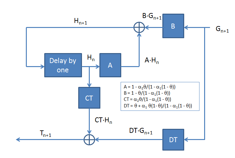 |
| Block diagram of system showing a single output ("measurement") variable T (the others (Y,YD,C) being similar) |
 |
| Discrete and continuous time system equivalents, where H[n] = h(n*Ts), etc. Ts being the sample period |
Notes:
[1] Note that another way to think of it in SFC discrete time model terms is that the inputs and outputs are not rates (like they are for the continuous time case), but rather quantities during the interval Ts. Ramanan made mention of this more than once in his comments on Jason's posts. Again, this is something an engineer would not normally do: he wouldn't change the interpretation from a rate to an amount just because he changed from continuous time to discrete time or vice versa. That'd be like changing from amperes to coulombs. But I guess the moral is that when playing with SFC models, do as the SFC modelers do!
[2] For convenience I'll reproduce Jason's comment about restrictions on alpha1 and alpha2 here:
In order to take larger time steps, you need to *increase* the value of alpha2. Unfortunately, alpha2 is restricted to be less than alpha1 by the model (and both must be less than one).
See Eq. (3.7) in Godley and Lavoie.
The values of alpha1 and alpha2 are later constrained in the text such that
(1- alpha1)/alpha2 = 1
called the "stock-flow norm".
It's a totally incoherent way to deal with the changes induced by changing the time step -- it violates the model assumptions and the rest of the analysis in G&L.
[3] Parameters expressions, reprinted here for convenience:
| Matrix | Element | Name | Expression | |||
| Ad | (1,1) | A | 1-theta*alpha2/(1-alpha1*(1-theta)) | |||
| Bd | (1,1) | B | 1-theta/(1-alpha1*(1-theta)) | |||
| Cd | (1,1) | CY | alpha2/(1-alpha1*(1-theta)) | |||
| (2,1) | CT | theta*alpha2/(1-alpha1*(1-theta)) | ||||
| (3,1) | CYD | (1-theta)*alpha2/(1-alpha1*(1-theta)) | ||||
| (4,1) | CC | alpha2/(1-alpha1*(1-theta)) | ||||
| Dd | (1,1) | DY | 1/(1-alpha1*(1-theta)) | |||
| (2,1) | DT | theta/(1-alpha1*(1-theta)) | ||||
| (3,1) | DYD | (1-theta)/(1-alpha1*(1-theta)) | ||||
| (4,1) | DC | 1/(1-alpha1*(1-theta)) - 1 | ||||
where the "d" subscript indicates "discrete time."
Nice, Tom!
ReplyDelete