SIM2: Interactive spreadsheet implementing Godley & Lavoie's SIM model (now w/ sample period invariance! [Hint: the secret is expm(A*Ts) & its integral have Ts parameters!])

tl;dr version: Everything you need to know is right here (except when A is singular, in which case you'll need this too to find discrete time B) which tells you about converting back and forth from continuous to discrete time in a problem like this, namely, given the system:

dx/dt = A∙x + B∙u       

for vectors x(t) and u(t) and constant matrices A and B and u(t) held constant over each sample period T, we have the discrete time equivalent:

Notice that the discrete time constant matrix coefficients Ad and Bd are dependent on the sample period T.

end tl;dr

Success!! (I think). I changed my previous spreadsheet to make it truly invariant to the sample period (Ts in the green box below). Please refer to the previous version and the description underneath the spreadsheet for what the formulas are doing and the discrete time state space representation of the system, and to links to Jason and Ramanan's blogs (from whence this whole exercise originated). Below the spreadsheet on this page I describe what I'm doing differently. Feel free to play with the values: I only planned on people editing the green cells (in this embedded version), and if you get it irrevocably screwed up, just refresh the page (you can't hurt my original copy). Also you can download your own copy using the tool on the right side of the black toolbar running along the bottom of the sheet. Note that setting Ts < 0.1 will limit the data to less than 100 years (so the plot won't be filled out) because the number of time samples in my table is fixed at 1000.

Note the names and values with the modifier "alt" in them below don't affect anything: they're part of an experiment to get SIM2 to always satisfy all of G&L's accounting expressions. I've had success with the ΔH = G - T expression by using T-alt (in columns to the right, you have to scroll to see). I did add T-alt to the plot so you can see how it differs slightly from T. More in Update 5 below and here.

NOTE (update of 2016.04.22): in the above sheet to calculate the so-called experimental "alt" version of values use CTalt = (1-A)/Ts and DTalt = (Ts-B)/Ts and alpha2alt = CTalt/DTalt, where A and B are a function of the new sample period Ts (assuming the old one Ts0 = 1). These expressions come from T as a function of Ts := T(Ts) = T*Ts = G(Ts) - ΔH(Ts) = G[n]*Ts - H[n](Ts) + H[n-1] = G[n]*Ts - A*H[n-1] - B*G[n] + H[n-1] = (1-A)*H[n-1] + (Ts-B)*G[n] = CTalt*H[n-1] + DTalt*G[n], assuming H[n-1] didn't change with Ts, and that A and B are functions of Ts, and that B requires multiplication by G expressed in old units (i.e. per Ts0). Then our new T expressed in old units as a rate (i.e. dollars per Ts0) is just T = T(Ts)/Ts = ((1-A)/Ts)*H[n-1] + ((Ts-B)/Ts)*G[n], thus matching terms  we have  CTalt = (1-A)/Ts and DTalt = (Ts-B)/Ts, and because C/D = alpha2 (where C is Cm, not SIM's consumption output C), then alpha2alt = CTalt/DTalt. I think the idea came from SIM3. Also see SIM5. Talt is calculated in terms of CTalt and DTalt in the columns you need to scroll to the right to see. The alpha2alt isn't actually used for anything (I don't think). It's a given that this experiment will "work" and that Jason's Γ = 1 for all Ts (the purpose of the "experiment"), given that we could just directly calculate Talt from the other columns: namely Talt = G - ΔH/Ts where the Talt and G columns are expressed as dollars per Ts0. Thus ΔH/Ts is just ΔH expressed in those same units. But ultimately the alpha2alt I calculate here doesn't lead anywhere. In contrast, SIM6 is a successful approach: it adjusts both alpha1 and alpha2 (but not theta) to change sample periods without affecting steady state values (expressed in dollars per Ts0 and in dollars for the case of H) or the time constant Tc (expressed in Ts0). An update there of the date of this update explains why you adjust alpha1 and alpha2 but not theta to accomplish that. Given that Ts is changed by changing these parameters, then it's a given that Jason's Γ = 1 for all Ts in SIM6 as well. That's not really the case here in SIM2 because the resultant alpha2alt is not used (because there's probably not a way to make it useful). Thus really Jason's Γ ≠ 1 for all Ts here (i.e. using the method here to change sample  periods). And no, alpha2alt here is not equal to the alpha2 from SIM6. However, that's not to say that the SIM3 idea didn't ultimately lead to a greater success: see SIM9  and SIM10  for example.

The problem with my previous sheet was that the H curve changed when I changed the sample period (Ts). This was in spite of modifying the alpha2 parameter as per Ramanan's instructions.

I've changed tactics here: instead of scaling alpha2 (from a user provided alpha2_R parameter), I instead just use the User Parameters (in the green cells) directly without doing any modifications, (e.g. modifications such as scaling alpha2 by the ratio of change in the sample period (Ts/Ts_orig)).

What I do instead is record the original Ts setting (Ts_orig = 1 years). Then from the alpha1, alpha2 and theta parameters I derive continuous time parameters for the system. In particular I do the following:

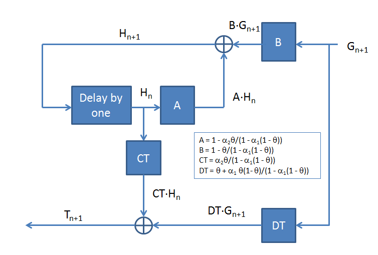
Starting with the original discrete time system with A_orig and B_orig based on alpha1, alpha2 and theta, we have:

H[n+1] = A_orig*H[n] + B_orig*G[n+1]

From this I calculate the parameters for an equivalent continuous time system assuming G is held constant over each sample period:

dH(t)/dt = H'(t) = a_cont*H(t) + b_cont*G(t)

From this continuous time system, I re-descretize it with a new sample period (the user input sample period Ts in the green cells in the upper left). This gives me a new A and a new B, which I simply call A and B like in the old spreadsheet, and use them as follows in the results table:

H[n+1] = A*H[n] + B*G[n+1]

Here's how I do the calculations. First I assume the A_orig and B_orig resulted from a discetization of a continuous time system with an original sample period Ts = 1 year (Ts_orig = 1). Thus:

A_orig = expm(a_cont*Ts_orig) = exp(a_cont*Ts_orig)  (matrix exponentiation expm() reduces to scalar exponentiation exp() in this case, since the system has a single state).

B_orig = (A_orig - 1)*b_cont/a_cont  (to see why this is, look here).

I solve for a_cont and b_cont from the above, and then use these same formulas with a new sample period (Ts) to calculate A and B.

Some of these calculations are performed in the cells to the right of the chart, and the rest are in the cells for the A and B matrices respectively.

Matrices C and D (used for calculating the measurement vector [Y T YD C]' at sample n+1 by scaling H[n] and G[n+1] respectively), were not changed.

Now (you may notice) instead of H changing with Ts, ΔH changes with Ts. Is that a problem? I don't think so, because it SHOULD change with Ts: each Ts period of time now adds less to the total stock of money in the economy. H should NOT be changing with Ts, because the sample period should not affect the total stock of money accumulated in the economy at a fixed time in years.

--------------------------------------------------------------------------------------------------------------------------- 
Further information about calculating A and B as a function of Ts/Ts_orig: 
 DoΔ Δ
Starting with A_orig and B_orig and doing a little algebra reveals:

(1) A_orig = A(Ts_orig) = 1 - theta * alpha2 / (1 - alpha1 * (1 - theta))

(2) B_orig = B(Ts_orig) = 1 - theta / (1 - alpha1 * (1 - theta))

I write A(Ts_orig) and B(Ts_orig) because they are implicit functions of Ts_orig! Equations (1) and (2) were our starting point for A and B on the previous spreadsheet. Now what happens when we change Ts_orig to Ts?:

(3) A(Ts) = A_orig^(Ts/Ts_orig)

(4) B(Ts) = (B_orig/(A_orig - 1)) * (A(Ts) - 1) = -[(1 - alpha1*(1 - theta) - theta)/(theta*alpha2)] * (A(Ts) - 1)

Note: I didn't bother with that algebra in the spreadsheet above: I just used exp() and ln() according the the development above equation (1).

Enjoy!

UPDATE 1: March 6, 2016 1:02 AM
I made a few changes to the plot to eliminate apparent sensitivity to Ts. Basically two things: I start the plot at t=0 years, but I start the table at -Ts. Secondly, instead of plotting H (which I leave in the main table), I plot H[n-1] (H delayed by one). H[n-1] takes the place of x[n] in a normal (canonical) discrete time state space formulation, so I suspected that I was plotting the wrong sequence against the others (off by one), and sure enough, once I changed that it helped quite a bit. The plot now shows near complete Ts invariance, as it should.
UPDATE 1: END

UPDATE 2: March 7, 2016 9:06 PM
Note that I resolved my problem with the old method of changing sample periods suggested by Ramanan on that older post, and I've updated it accordingly (read Update #2 there at the top). However that doesn't mean that the alpha2 scaling method is the same as this method: it is for small values of Ts, but try Ts >= 10 on this sheet and that one to see how they still differ.
UPDATE 2: END

UPDATE 3: March 8, 2016 12:33 AM
Note the  Γ below is Jason Smith's Γ from his March 2016 posts on SIM.

UPDATE 3: END

UPDATE 4: March 9, 2016, 5:21 PM
I made a new version called SIM3 posted here which combines the best of the version above (SIM2) with the old version (SIM), for the price of restricting the functional form of G.
UPDATE 4: END

UPDATE 5: March 13, 2016, 2:50 PM
I added some "alternative" parameters and variables to the spreadsheet. They don't affect any of the previous parameters or the plot, except that I've plotted T-alt to the plot. It differs slightly from T when Ts is changed. T-alt satisfies G&L's ΔH = G - T (actually ΔH = Ts*(G - T) since G and T are always rates expressed in dollars/(Ts_orig = Ts1 = 1 period = 1 year) in SIM2). Eventually there will be alternate versions of theta (thetaalt) and alpha1 (alpha1alt) as well. The idea is to eventually satisfy ALL of G&L's accounting equations, while maintaining sample period invariance, and matching G&L at Ts=1 (at least with G functions restricted to the form of their example). I have more information about it under the heading "SIM5" on a new post called SIM5.
UPDATE 5: END

UPDATE 6: March 17, 2016, 10:17 AM
As I explain in a new post (SIM6), and in a comment on Jason's blog, think Jason's Γ (above) represents both an approximate change to a new sample time (without actually changing the sample time values in the table), thus a time constant change without a change in steady states (what I explain in the comment). And, as I explain in the text of SIM6 below the spreadsheet) Jason's Γ as calculated above represents the difference between a sampled rate variable (like I treat G, Y, T, YD and C in the spreadsheet in this post) and an average rate calculated across a sample period interval (how they are treated in SIM and SIM6). As Ts gets larger, that difference grows.
UPDATE 6: END

SIM: Interactive spreadsheet implementing Godley & Lavoie's SIM model (with "approximate" sample period invariance)

UPDATE 1: March 5, 2016, 3:36 PM
I think I solved the problem with changing the sample period Ts I describe below, but rather than edit this spreadsheet (which highlights the problem pretty well I think), I created a new spreadsheet in a new blog posting here.
END UPDATE 1.

UPDATE 2: March 7, 2016, 8:04 PM
I think I solved the problem with changing the sample period Ts on this sheet after receiving this comment from commenter "A H" on Jason's blog. I realized that when stock-flow consistent (SFC) modelers put together their model there's a difference in philosophy compared to how an engineer putting together a discrete time state space finite difference model approaches it. The engineer does NOT in general want the units of his exogenous inputs and outputs (output AKA "measurements") to change simply because he's chosen a new sample period (Ts). In contrast the SFC modeler assumes they change to match the new time scale [1]. For example, G&L use a sample period of 1 (which I call a "year" to give it a name). I call this Ts_orig and its value is fixed at 1. Ts is the sample period actually used (a user input) and it's therefore measured in years. So Ts = 2 means 2 years, etc. Thus when I change Ts I now scale the numerical value of the exogenous input by Ts/Ts_orig to express it in dollars/Ts and I interpret the outputs Y, T, YD and C as if they are expressed per Ts (rather than per Ts_orig). These rates have not changed, but the units they are expressed in have. This fixes the biggest problem I had before with Ramanan's suggested method of just scaling alpha2 by Ts/Ts_orig to change sample periods. He naturally thought I'd be changing units on G and interpreting the outputs as if they'd changed units as well, when from a state space perspective (which is the framework I used to construct this model) that would never be done. This fix required adding a new results table in which the results are actually calculated with scaled alpha2 and G expressed in new units. You have to scroll out to the right to see this new table. The results are scaled appropriately and copied back to the old table, from whence the plot is made. Note that I have now applied the same fixes to the plot here that I did in my next post using a different method for changing sample periods (see Update #1 above).

"Approximate" results with alpha2 scaling:
The only other issue is that scaling alpha2 by Ts/Ts_orig produces results which are an approximation of sampling an equivalent continuous time system. Or put differently, when Ts changes, the equivalent continuous time system changes. The difference in this case is pretty small until you get out to Ts >= 10, in which case you can see it start to break down. The results may still be SFC, but they are no longer samples of the same underlying continuous time system which Ts=1 were samples of. Try it out and see: if you set Ts = 10 in the green box below, the system starts to "ring." Another way to think of this is the compounding is no longer a good approximation to continuous compounding. To avoid these kinds of problems (if indeed it is a problem for you, it may not be), make sample period adjustments as I describe in my next post, and the continuous time system you'll be sampling will be independent of the sample period. Try it out: set Ts=10 on the spreadsheet on that post, and you'll continue to get samples from the same rising exponential, without any ringing. I have not done a careful analysis, but I suspect that's what's going on.
END UPDATE 2.

UPDATE 3: March 7, 2016, 10:24 PM
Regarding setting Ts to large values, Jason Smith has pointed out an important point [2] regarding G&L restrictions on the values of alpha2 and alpha1, so the method of scaling alpha2 can really only be used for Ts < Ts_orig*alpha1/alpha2. With alpha1 = 0.6 and alpha2 = 0.4 originally, that means Ts <= 1.5.
END UPDATE 3.  

UPDATE 4: March 9, 2016, 5:23 PM

I've got a new version (SIM3) which still matches G&L at Ts=1, is completely Ts invariant, and always satisfies ΔH = G - T. The downside is the functional form of G is restricted to a scaled step (as it is in G&L's example).

END UPDATE 4.  

UPDATE 5: March 15, 2016, 10:00 PM

SIM6 is a direct replacement for this spreadsheet: it adjusts both alpha1 and alpha2 to preserve both the time constant (thus achieving sample period invariance), and satisfying all G&L's expressions.

END UPDATE 5. 
 
 



More information here on Jason Smith's blog post:
http://informationtransfereconomics.blogspot.com/2016/03/more-like-stock-flow-in-consistent.html

Note that the difference equation implemented in the table (under the chart) is:

Difference equation:
H[n+1] = A*H[n] + B*G[n+1]

Measurement equations:
Y[n+1] = CY*H[n] +  DY*G[n+1]
T[n+1] = CT*H[n] +  DT*G[n+1]
YD[n+1] = CYD*H[n] +  DYD*G[n+1]
C[n+1] = CC*H[n] +  DC*G[n+1]

Which is not quite standard discrete time space space representation (normally the index on H (normally called the state vector x) and G (normally called the input vector u) would match instead of be off by one in relation to each other), but I wanted my table to match Jason Smith and Godley & Lavoie, at least in terms of the contents across one row (columns in their cases). Also, in the table, I subtracted one sample period (Ts) from my time index in relation to theirs so I could start at 0 rather than Ts. The purpose of this is to cause less disruption on my plot should the Ts user parameter be changed.

Also note that with the default parameters, this model works as expected and reproduces the results of Godley & Lavoie (just as Jason Smith's model does), but a secondary purpose was to test the idea of changing the sample period (Ts). Ramanan notes in comments on Jason's post an on his own blog post on this subject that doing so requires a change in alpha2. That's why I introduced the alpha2_R parameter and have a separate alpha2 which is adjusted by Ts in the manner Ramanan suggested (I think!). Most of the curves do seem to be invariant to a change in Ts with this adjustment made to alpha2, except for the H curve. So I need to find out why. See my Update #2 at the top: I now know why, and have fixed this sheet.

Block diagram of system showing a single output ("measurement") variable T (the others (Y,YD,C) being similar)

Discrete and continuous time system equivalents, where H[n] = h(n*Ts), etc. Ts being the sample period

Notes:
[1]  Note that another way to think of it in SFC discrete time model terms is that the inputs and outputs are not rates (like they are for the continuous time case), but rather quantities during the interval Ts. Ramanan made mention of this more than once in his comments on Jason's posts. Again, this is something an engineer would not normally do: he wouldn't change the interpretation from a rate to an amount just because he changed from continuous time to discrete time or vice versa. That'd be like changing from amperes to coulombs. But I guess the moral is that when playing with SFC models, do as the SFC modelers do!

[2] For convenience I'll reproduce Jason's comment about restrictions on alpha1 and alpha2 here:

In order to take larger time steps, you need to *increase* the value of alpha2. Unfortunately, alpha2 is restricted to be less than alpha1 by the model (and both must be less than one).

See Eq. (3.7) in Godley and Lavoie.

The values of alpha1 and alpha2 are later constrained in the text such that

(1- alpha1)/alpha2 = 1

called the "stock-flow norm".

It's a totally incoherent way to deal with the changes induced by changing the time step -- it violates the model assumptions and the rest of the analysis in G&L.

[3] Parameters expressions, reprinted here for convenience: 

Matrix	Element	Name	Expression
Ad	(1,1)	A	1-theta*alpha2/(1-alpha1*(1-theta))
Bd	(1,1)	B	1-theta/(1-alpha1*(1-theta))
Cd	(1,1)	CY	alpha2/(1-alpha1*(1-theta))
	(2,1)	CT	theta*alpha2/(1-alpha1*(1-theta))
	(3,1)	CYD	(1-theta)*alpha2/(1-alpha1*(1-theta))
	(4,1)	CC	alpha2/(1-alpha1*(1-theta))
Dd	(1,1)	DY	1/(1-alpha1*(1-theta))
	(2,1)	DT	theta/(1-alpha1*(1-theta))
	(3,1)	DYD	(1-theta)/(1-alpha1*(1-theta))
	(4,1)	DC	1/(1-alpha1*(1-theta)) - 1

where the "d" subscript indicates "discrete time."

Algebra Part 1

Starting with Jason's second expression here:


$$\frac{J}{J_{ref}}={\left(\frac{L}{L_{ref}}\right)}^{1/\mathrm{\kappa <!--\; \kappa \; -->}}$$


Raise both sides to the (κ - 1)th power:


$${\left(\frac{J}{J_{ref}}\right) }^{\mathrm{(}\mathrm{\kappa -1)<!--\; \kappa \; -->}}={\left(\frac{L}{L_{ref}}\right) }^{\mathrm{(}\mathrm{1-1/\kappa )<!--\; \kappa \; -->}}$$


Now divide both sides by the right side:


$${\left(\frac{J}{J_{ref}}\right)}^{\mathrm{\kappa <!--\; \kappa \; -->}-<!--\; -\; -->1}{\left(\frac{L}{L_{ref}}\right)}^{\mathrm{}<!--\; -\; -->1/\mathrm{\kappa \; -\; 1<!--\; \kappa \; -->}}=1$$

Scott in Hell

Getting all caught up on every MF lecture he ignored...

 ...FOREVER!   Mwha-hahahahaha!

Nick Edmonds' simulation model for Samuelson and inside money: interactive version

Here is an updated interactive sheet. Six iterations are done now at each time step and I've produced all the plots. If you download the spreadsheet you'll see all the calculations are done on a single page now. Instead of parameter "gL" entered as a percentage (like I had before) I kept it as factor "g" so for example instead of entering 2% you'd now enter 1.02. I did this just to be consistent with Nick Edmond's blog post. I kept my original blog post here underneath this new spreadsheet. Enjoy! (There may be a bug: this one is not as robust as the old one: it doesn't handle changing in the inflation rate very well: but on the plus side you can try changing some of the other parameters). I corrected one bug: the solution always started from the same initial guess when it should have used the solution for the time step before as the first guess, thus it didn't always converge: Newton's method (in this case the vector version) is sensitive to where you start: you need to be close enough (in which case it converges rapidly), which you can get a feel for here. But I still have a problem with the auto-scaling of the plots. I think this is because I'm plotting values across hidden rows. The values in the hidden rows are not plotted, which is what I want, but I suspect they still do contribute to the axis auto-scaling solution. This problem is only apparent in the Price of Land plot with the default input parameters, but becomes apparent in other plots when you change some of the other parameters. The "eps" parameter only affects the Newton's method solution (it's the size of perturbations used to numerically calculate the Jacobian matrix) and has nothing to do with the model, but you can change that too (note in this case the Jacobian could well be calculated in closed form, but I wanted a more general approach). I have not tried changing all the different parameters, so it's quite possible you could break it! I've mostly just played with "g" and "alpha."





I never did end up using the circular reference iteration facility in Excel because of the nature of this problem: each time step depends on the prior one. Thus you can't really iterate at each time step independently. Thus the iterations are hardcoded in the spreadsheet, but in a fairly compact fashion. If you try downloading the spreadsheet, the "Results" sheet does all the work and looks fairly tidy, with the solution at each time step laid out one per row in a table. If you were to unhide all the rows and columns however, it would look worse, but not unmanageable. Between each pair of rows (save the 1st two), are the six Newton's method iterations laid out with the solutions in columns (I transpose to save vertical space). It's set up in such as way that if you want to add time periods, you can just copy and paste these unhidden blocks to the end (so, for example, it'd be easy to nearly double the number of time steps with a single copy and paste of the existing solution blocks appended to the end). Unhiding all the cells is not obvious, but only because I hid cell A1. Unhide that one and you're good (I'll let you figure that out... you may need to do some Googling). In fact, probably unhiding is not necessary to simply extend this solution to more time steps: simply copy paste rows of the existing table to the end. You'd need to adjust the plots of course. But if you want to see how it works or change the formulas, then you need to unhide.

Here's an update to the above. You can indeed keep the spreadsheet looking tidy and use a copy and paste procedure to extend the solution to more times, but doing this is not completely obvious, so I'll give some instructions here. The problem is a straight copy and paste leaves out some of the hidden cells at the top which allows the solution to propagate forward to each subsequent time. To get around this problem you need to unhide at least one of the hidden rows. First go to the "Results" tab of the downloaded spreadsheet. The cells implementing Newton's method are not present between times 0 and 1 (though unlabeled, time is in the 1st columns of the table on the left on the results page). You *could* just unhide all the hidden rows and columns, but to keep it looking tidy and to make it easier to work with we'll just unhide the first row after the time = 1 row, which at the time of this writing is row 4. Use the instructions here (I'm solving the puzzle I proposed you solve yourself with Google in the above paragraph, except on row 4 instead of cell A1). To do this for row 4, replace "A1" in those instructions with any hidden cell in the spreadsheet under row 1 that you'd be able to see if all rows (not columns) were unhidden. So for example the one on the far left of the unhidden columns in row 4 should work: as of this writing, that would be cell "E4." Following the instruction on the link, select "unhide row" in the drop down box on the format menu. Now you should see a blank row appear between the time = 1 and time = 2 rows: in this case row 4, starting with cell E4 on the left. Now copy the full rows starting with row 4 down to however many times you want to add. If you want to add 5 new times, copy from row 4 to row 108 (keep in mind there's a lot of hidden rows in between, which is why the end row is not row 9 = 4 + 5 here), then paste them starting in the first row beyond the bottom of the table (row 403). Be sure to select that whole blank row (row 403) to paste into, otherwise it won't let you do the paste operation, as depicted in Figure 1. Also note in Figure 1 the dashed green outline near the top showing the cells selected to copy. Column W separates the results table on the left from the charts data table on the right (only two columns of which are depicted).

Figure 1: Screenshot of spreadsheet just prior to pasting the copied rows

You should see the block of rows get filled in with answers. The times in the far left column should now range from 21 to 25 in the new rows. This is depicted in Figure 2. Notice how the 1st column on the left (time) started not with 2 (the time in the copied row 4) but with 21 (the first time past the last time entry in the existing table).

Figure 2: Screenshot of spreadsheet immediately after pasting the copied rows.

Now you can continue to paste more cells until you get the table extended out to the time you want. Finish up by re-hiding all the blank rows in the results table. You'll notice that you get some bad values in the table to the right of the results table (in the otherwise blank rows): that's the chart data table for the charts on the "Parameters" sheet. Ignore those: once the row is hidden you can make new charts by either creating them from scratch or updating the data series in the existing charts to include the new rows: the bad values in the hidden rows should not get plotted. You'll need to reformat the x-axis of the chart(s) too because I fixed the maximum value at 20. Good luck!

Below is my original post which I'll leave intact for now:

 

From Nick Edmonds' Simulation Model for Samuelson and Inside Money post. You can edit the whole workbook. If you mess it up and want to start over, just reload the page. This is a first attempt at doing this kind of thing online iteratively with free online spreadsheets. I think I may be onto a better approach here, but have yet to connect all the dots. The "Growth rate for nominal loans" cell at the top changes the gL variable in Nick's write up (see this comment). Nick actually discusses the "Growth parameter for nominal loans (g)" in his table of variables, but the relationship is simple: g = 1 + gL. Enter it as a percentage in the long orange cell near the top (A2:E2). The workbook iteratively solves the equations, but only two iterations are used for each point in time. Check the columns "Cw err," "pa err" and "pc err" to see how close to a solution the two iterations get you. You may need to use the scroll bars. You should see the plot change when you change gL. It's definitely not perfect, but it should work reasonably well for values of gL near 2%.

Newton's method: a forward difference is used to calculate a Jacobian to solve the problem and "delta_base" is the size of the perturbation to the Cw, pa, and pc variables at each time (Each year is a row in the spreadsheet). You can change "delta_base" by editing cell F2 (dark gray) just to the right of gL. The solution shouldn't be too sensitive to delta_base. I could improve the solution by adding more iterations to each of the other tabs labeled 2 through 21. These sheets are a bit ugly... I was interested in getting it to work online with minimal effort (Excel "Solver" and macros are not available online). You can download the workbook by clicking on the Green "X" Excel symbol on the right hand side of the black bar across the bottom of the spreadsheet.

Nick Rowe's example from 'The sense in which the stock of money is "supply-determined"'

Figure 1: Diagram of Nick Rowe's example

In a post from Nick Rowe regarding the sense in which the stock of money is "supply-determined" he sketches out an example with the following definition for the money demand function:

Md=L(P,Y)=PY

He also mentions that:

By cutting the rate of interest, the central bank increases the quantity of loans from the central bank, which creates more money. Eventually P and/or Y will increase and the quantity of money demanded will increase in proportion to the quantity created.

Figure 1 is my attempt to sketch out what this example looks like. The items with "0" indicate the original values prior to the central bank's exogenous cut in interest rates from r0 to r1. Keep in mind that the central bank (CB) is the ONLY bank in this example: there are no commercial banks, and it only loans cash (so no deposits at all in this world) and it is compelled to lend to anyone because they are all good credit risks. I'll also assume that the bank is compelled to sell back to each individual borrower their debt on a dollar for dollar basis at the discretion of the borrower. Some of these assumptions may not be important for the logic of the post though!

Note that the blue downward sloping curve in the upper plot is the "supply curve for loans determined by borrowers" which Nick states is equivalent to "demand for loans by borrowers" in "normal language." He points this out in the comments in his previous post. Also note Md0 corresponds to Y0 and Md1 corresponds to Y1 (if P did not change from P0). However, it's possible also that Y does not change from Y0 and P instead changes from P0 to P1. In fact Nick implies that either or both P and Y could increase in this case which gives us the set of solutions for 1/P lying between the two blue money demand curves (Md0 and Md1) along the red supply curve on the right (Ms1).

Scott Sumner thinks that Nick must mean that where Md0 and Ms1 cross is the solution. He also claims that the MMT people would say that the solution is where Md1 and Ms1 cross. I think Nick is actually saying it can lie anywhere between those extremes.

Also note that in the upper plot the two horizontal green solid lines are the "perfectly-elastic supply functions" for money (each at a fixed interest rate, r0 and r1), and that the two vertical red lines in the upper chart are the two "perfectly interest inelastic" demand curves for  money. Assume the red vertical line on the left is Md0 and that it has already reached equilibrium to match the supply of money (Ms0 in the lower chart). After r is lowered from r0 to r1, then Ms0 goes to Ms1 in accordance with the borrower determined supply for loans curve in the upper plot. Then *eventually* the demand curve for money in the upper plot (still perfectly interest inelastic, and thus vertical) will move right to match the supply curve (Ms1) in the lower plot.

One more thought on the upper plot (with the CB "exogenously" determined interest rate on the y-axis). The solution where the downward sloping blue curve (borrower determined supply curve for loans) intersects the horizontal green "perfectly interest-elastic 'supply' curves for money." I've already noted how in "normal language" (according to Nick) the "supply curve for loans" is called "demand for loans." However, it's better described as a supply curve. But then we have two supply curves intersecting. But then it occurred me to make the following linguistic substitutions, and I think it all becomes a lot more clear:

Replace "loans" with "bonds."
Replace "borrowers" with "bond issuers."

Then the blue line's name makes more sense as a supply curve as we've noted. But also, the horizontal "supply for money" curves instead become "perfectly interest-elastic *DEMAND* curves for bonds at exogenously fixed rates of interest." So then we're back to quantity being determined in the usual way by a supply curve intersecting a demand curve. Hurray! I comment on that here on Nick's post.

The red perfectly interest-inelastic vertical demand for money curves in the upper plot do NOT determine the quantity of money, and instead follow the solution determined by the other two curves.

Note: Scott Sumner suggested in a comment that instead of 1/P on the y-axis in the lower plot, I should instead plot 1/NGDP = 1/(P*Y). If I did this, then there would only be a single downward sloping (rectangular hyperbola) blue Md curve and the solution set of Nick Rowe at Ms1 would collapse to a single point on that curve. I.e. Scott's solution and the "MMT" solution would be indistinguishable (which would probably not please Scott!).

Note that in the upper plot, the x-axis could be labeled "Quantity of loan-principal demanded/supplied (measured in dollars)."

With this later comment, Nick Rowe essentially establishes his solution set at r1 (in Figure 1's lower plot) to be the entire red ray labelled "Ms1"... it would be the small line segment if P and Y were precluded from decreasing.

Nick Rowe vs Scott Sumner: Different Answers to a Simple HPE Hypothetical

Figure 1: Nick Rowe's and Scott Sumner's solutions for P

This is a simple hypothetical that I feel get's to the core of concepts like the long term neutrality of money, the quantity theory of money (QTM), and the hot potato effect (HPE) which undergird much of Market Monetarist (MM) thought. If I'm not mistaken, Nick Rowe seems to think my hypothetical is a case where those concepts don't work, while Scott disagrees. Why do I care? Well if they don't work here, then what about our real situation does make them work? How can we be certain that they are indeed working, and if they are how do we know they are completely working?

Setup: This is basically the same as Scott Sumner's "cashless society" hypothetical (case 7) except with the added stipulation that there's just one commercial bank and that the reserve requirement is 0% (Scott didn't specify the number of commercial banks or the reserve requirement). In particular, we have:

1. Cashless society (no paper reserve notes and no coins).
2. A central bank (CB) which can buy and sell assets (open market operations (OMOs)).
3. A single commercial bank with a CB deposit (i.e. reserve deposit). This is the only existing CB deposit account.
4. The reserve requirement is 0%.
5. A non-bank private sector which holds deposits at the commercial bank.

Scott points out that in such a case base money consists only of bank reserves (as there's no cash) and thus reserves alone are the medium of account (MOA)*. Now for some important definitions:

P = average steady state price level in the private economy
Ms = reserve supply
Mdn = nominal reserve demand
Mdr = real reserve demand = Mdn/P

Scott Sumner and Mark A. Sadowski say that if Ms changes (e.g. through CB OMOs), then P will change in proportion. Nick Rowe says that in this case demand for reserves will change with Ms. Specifically he noted that if Ms goes to zero then demand for reserves will go to zero. If we take this to mean that demand is proportional to Ms, then P stays fixed regardless of the change in Ms.

The difference between Nick's and Scott's solution is illustrated in Figure 1 for two different values of Ms: we're assuming they start off the same at Ms = Ms0, but then the CB sells assets such that Ms = Ms1. The demand curve (Mdn) in Nick's case scales in proportion to Ms (this is accomplished by scaling Mdr). Nick Rowe says that my Figure 1 looks roughly right. Click here to see an animation.

My question for Nick is what is preventing the long term neutrality of money in this case? What would I need to change about my example, aside from adding cash, for him to agree with Scott? For example, would adding multiple commercial banks do it? Something else? What's the minimum change required?

Relating my hypothetical back to reality, is it really so outlandish to consider the case of a single commercial bank? Mark Sadowski identified a case in France in which the banks were nationalized, and he notes with little effect. In terms of a cashless society, Mark is convinced we'll still have cash a hundred years from now, but Scott agrees it is going away at some point. I believe Canada looked into the consequences of going cashless. But even if Mark is right and cash is here for the long haul, does it really make much of a difference? Isn't it just an arbitrary choice by the depositor about which form to keep his money in? (Mark & Mishkin agree it's the "depositor's choice.") Does it really affect the long term neutrality of money, the QTM and the HPE?

*Although only reserves are MOA, I think both Scott & Nick would agree that both reserves and commercial bank deposits are a medium of exchange (MOE) in this case.

For those wishing to see the above change in Ms sketched out in balance sheets, look here.

Additional notes and links can be found here (warning: redundant and unorganized!)

Although I compiled a more succinct history of this question here, (a copy here) and the question itself has been brought up again here and here. Also, I discuss the history of a preceding related question here (in which the CB buys up the commercial banks).